Due to overwhelming demand, I figured I should make more of an introductory post about some of the motivations for reinforcement learning and introduce some basic terminology, which I will be using throughout the rest of this blog series. I’ll try to keep this post relatively accessible but I do assume at least a basic understanding of machine learning and statistics. Alright then, without further ado, let’s get started!
Inspirations
:max_bytes(150000):strip_icc()/2794863-operant-conditioning-a21-5b242abe8e1b6e0036fafff6.png)
Reinforcement learning is an approach to machine learning, which is concerned with goal-directed behavior. The types of problems that reinforcement learning tackles are very different from the other two more common paradigms of machine learning, which are supervised and unsupervised learning. Specifically, the goal of reinforcement learning is to derive the optimal policy or pattern of behavior for a control problem.
This paradigm is heavily modeled after biological systems and reward-based learning found in psychology. In fact, the pioneer of reinforcement learning, Richard S. Sutton, did his undergraduate degree in psychology and not computer science (although I don’t really recommend this if you want to purse a job outside academia). In fact, many of his high-level ideas can be traced back to operant conditioning, which is an idea that behavior can be influenced with rewards and punishments.
Multi-armed bandits
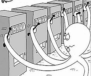
To concretely illustrate the type of problem that reinforcement learning attempts to solve, let’s go through a popular example and gradually build upon it. Imagine that there are 


Now, what if those same reward probabilities are gradually changing with time (i.e. non-stationary). Well in this case, it would be wise to introduce the idea of discounting with a new parameter, 

So let’s continue by adding another wretch in the the traditional multi-armed bandit problem. Now imagine that the probability of getting a reward from each slot machine is changing dynamically after each play. In fact its changing so much that simply discounting the reward signal isn’t enough to come up with the best strategy. This means that every time you pick a slot machine, it’s like all of the previous machines are replaced with new ones; you’ve essentially arrived at a new state. The assumption now is that any immediate action taken impacts both the immediate reward along with the next state. In this case, the goal is to learn a policy, 
The RL Problem

Now that you have a rough idea of how this all works, let’s try to generalize these ideas a bit more. All reinforcement learning problems can be broken up into a series of states, 


This all seems simple enough until you take into account the credit assignment problem. That is, how does one properly assign credit to each action that one takes within an MDP? This is a difficult question to answer as many seemingly suboptimal actions taken at the current time step can have significant pay off later on. Many reinforcement learning algorithms attempt to back-up some of these reward signals and gradually learn more about the underlying dynamics of an environment through direct interactions with it. This is done by either incrementally iterating upon the value of a state following a certain policy, 

Another difficulty in reinforcement learning comes from addressing the exploration-exploitation problem. This problem deals with balancing the requirements of picking the best action with respect to the current knowledge of the environment or continuing to explore the state-space to come up with better actions in the future. This issue is especially tricky if the state space is very large or continuous. Many algorithms address this issue by introducing some stochasticity into the decision-making process or by using function approximators (i.e. neural networks).
By now you’re probably wondering, how do we solve these problems and where do they actually show up in the real world? Well, I’ll probably need a couple more blog posts to answer the first question but I’ll try to answer the second one in the next section.
Applications
The power of RL versus more classical methods for control comes from its generalizability and scalability when combined with neural networks. David Silver first proved this point by showing a deep RL agent perform above human capabilities on a number of classic Atari games (you can read more about it here). His research proved that reinforcement learning can be applied to many simple games to learn optimal behavior. However, the applications don’t end there. In fact, reinforcement learning can be applied to any decision-making process where the environment can be at least partially represented as an MDP.
Here are some more examples:
- A stock-trading agent that will improve its strategy for trading through experience alone (paper) or alternatively an agent that learns to trade specifically in cryptocurrencies (I can hear all the SV VCs fawning already)
- A RL agent that learns to adapt to difficult network conditions to deliver the best quality of experience for a user watching streamed video content (paper)
- A RL agent that acts as the flight controller for an autonomous helicopter (paper)
- A RL agents used to control a manufacturing robot that performs generalized automation tasks (paper)
I could go on but suffice to say, the applications of reinforcement learning are diverse and varied.
Conclusion
I hope this post has given you a gentle introduction to reinforcement learning. In the next couple of posts, I’ll be covering some foundational knowledge on RL along with some popular algorithms applied to some interesting problems. If there are any inaccuracies in this post or if you have general feedback for me, feel free to shoot me an email or leave a comment below 🙂
