Congrats on making it past the previous post. That last post was pretty theory heavy and covered a lot of ground on Monte Carlo Methods. For this blog post, I’m going to pick up the pace a little bit and cover some more fundamental RL algorithms. In fact, by the end of this post, you should have a decent theoretical and practical understanding of the Dueling DDQN algorithm. Again, I’ve gathered most of this information from reading research papers on DQN, watching David Silver’s RL course and reading Sutton and Barto.
Throughout this post, I’ll be building upon an implementation of this algorithm in python to give you more insight into the finer details. After every code snippet, I’ll try to explain some of the lines that may be difficult to understand or are key to the underlying algorithm. During these sections, I find it most helpful to open up this blog post in another tab and go through the code line by line with my explanations. I’ve adopted this methodology from Trask’s blog post on implementing neural networks with numpy (which by the way, I highly recommend going through if you’re serious about this stuff). Aside from that, you can be sure to find full implementations of any of the algorithms I discuss in this post and in my previous posts on my GitHub.
Q-Learning
So let’s begin with the vanilla Q-learning algorithm using simple table look up methods. How does this algorithm work? Well, Q-learning is a simple off-policy learning method based off of the idea of bootstrapping. Bootstrapping is the idea that new estimates can be made from previous estimates. This idea is different from Monte Carlo Methods (MCM), which were discussed in detail in the previous post. In MCM, the agent bases its policy updates on only the returns obtained from the most recent episode. However, in this case, the Q-learning algorithm performs policy updates after every step taken in the environment rather than all at once at the end of an episode. This means the algorithm is more adaptive to changes in the environment and less susceptible to the high variance involved with updating the policy on only a single experience trajectory. Q-learning along with all algorithms that use bootstrapping to perform the generalized policy iteration (GPI) technique are identified as temporal difference methods.
Mathematically, in Q-learning the updates to the Q-values are performed using Equation 1 while in MCM, the update operation looks more like equation 2. The key difference here is that with Q-learning, the update operation is applied online, when the entire discounted return from a specific time step (


Equation 1: Q-Learning Update

or equivalently,

Equation 2: Off-policy MCM Update

Another thing to notice here is that I don’t have to worry about importance sampling ratios (

Figure 1: Comparing MCM Updates (left) with TD updates (right) for decision-making. Taken from Lecture 4 of David Silver’s excellent introductory RL course.
Note: The above images uses 

Let’s see how this looks like in code.
def q_learning(env, num_episodes, discount_factor=1.0, alpha=0.5, epsilon=0.1):
    """
    Vanilla Q-Learning algorithm: Off-policy TD control. Finds the optimal greedy policy
    while following an epsilon-greedy policy

    Args:
        env: OpenAI environment.
        num_episodes: Number of episodes to run for.
        discount_factor: Gamma discount factor.
        alpha: TD learning rate.
        epsilon: probability of sampling a random action, a float value betwen 0 and 1.

    Returns:
        A tuple (Q, episode_lengths).
        Q is the optimal action-value function, a dictionary mapping state -> action values.
        stats is an EpisodeStats object with two numpy arrays for episode_lengths and episode_rewards.
    """

    # A nested dictionary that maps state -> (action -> action-value)
    Q = defaultdict(lambda: np.zeros(env.action_space.n))

    # The policy we're following
    policy = make_epsilon_greedy_policy(Q, epsilon, env.action_space.n)

    for i_episode in range(num_episodes):
        done = False
        s = env.reset()

        while not done:
            action = np.random.choice(np.arange(env.action_space.n), p=policy(s))
            new_s, r, done, _ = env.step(action)
            Q[s][action] += alpha * (r + discount_factor * np.max(Q[new_s]) - Q[s][action])
            s = new_s

    return Q
Some things to note here:
Line 23: the make_epsilon_greedy_policy function holds a reference to the Q table/function and returns a function (policy). This returned function when invoked, returns a probability distribution over possible actions in each state (
Line 33: Most of the magic for this algorithm happens in this line. If you carefully examine it, you’ll notice it’s exactly the same as Equation 1 from before.
Deep Q-Learning (DQN)
This all seems pretty reasonable right? But by now I bet you’re wondering where the deep in deep reinforcement learning come in. Before I get to that let’s go back to the previous algorithm for a bit and examine one its biggest flaws. What’s this flaw you ask? Well, imagine a problem with a million discrete states or a continuous state space. Now imagine training this algorithm in this environment and storing each of the state-action values. It doesn’t take a genius to realize that you’re quickly going to run out of memory without getting very far in the training process. So how do we make this algorithm more scalable? Well let’s add our favorite buzzword and mathematical blackbox, the neural network, into the mix. Brace yourself as we’re now entering deep RL territory.
The major difference here is that instead of querying a table to obtain the Q-value associated with each state-action pair, we’re going to be using a neural network to approximate it. This neural network will take the current state and output a set of Q values associated with each action that the agent can take in the current state.
However, there are still a couple of small changes we have to make to incorporate the neural network into the Q-learning algorithm. Specifically, we need to introduce the concept of a target network and experience replay to stabilize the training process. One of the major differences in the use of neural networks in reinforcement learning as opposed to supervised learning, is that the target output isn’t stationary. This is because as the agent explores the environment, it iterates on its policy and changes it’s Q-values accordingly. Moreover, training a neural network on such a highly non-stationary target would quickly lead to instability (imagine chasing a moving bus as opposed to a stationary one). To address this issue, many implementations of the Deep Q-learning (DQN) algorithm use two Q-networks. The first network is updated after every time step using back propagation as usual (the working network) and the other network is used exclusively to predict the TD target (the target network). In this case, the target network serves as a semi-stationary target as it is updated less frequently than the working network. Moreover, whenever the target network is updated, the update process simply involves copying the weights from the working network.
The other technique that’s used to aid in stability is experience replay. Experience replay is a technique where the agent explores the environment while maintaining a buffer of state transitions. This buffer of experience is then randomly sampled and the resulting samples are used to perform the generalized policy iteration. But why would anyone opt to do this instead of just using the most recent transitions? Well, that idea may work for tabular Q-learning, but it’ll likely lead to stability issues when non-linear function approximators like neural nets are used to learn the Q-function. These stability issues arise from multiple convergence proofs that require neural networks be trained on independently and identically distributed data (i.i.d. data). By training a model on continuous transitions, there exists strong correlations between samples, which clearly violates the i.i.d. requirement. This issue can be remedied by using experience replay and randomly selecting a batch of previous state transitions for training. Furthermore, this technique also enables the network to train on the same state transition multiple times, which aids in generalization.
So how does this all look like in practice? Let’s go through an implementation.
def deep_q_learning(sess,
                    env,
                    q_estimator,
                    target_estimator,
                    n_steps,
                    replay_memory_init_size=64,
                    epsilon_decay_size=1000,
                    replay_memory_size=10000,
                    update_target_estimator_every=100,
                    discount_factor=0.99,
                    batch_size=32):
    """
    Q-Learning algorithm for off-policy TD control using Function Approximation.
    Finds the optimal greedy policy while following an epsilon-greedy policy.

    Args:
        sess: Tensorflow Session object
        env: OpenAI environment
        q_estimator: Estimator object used for the q values
        target_estimator: Estimator object used for the targets
        n_step: Number of steps to run for
        replay_memory_size: Size of the replay memory
        replay_memory_init_size: Number of random experiences to sample when initializing the reply memory.
        update_target_estimator_every: Copy parameters from the Q estimator to the target estimator every N steps
        discount_factor: Gamma discount factor<span id="mce_SELREST_start" style="overflow:hidden;line-height:0;"></span>
    """
    # The replay memory
    replay_memory = []

    epsilon_start = 1.0
    epsilon_final = 0.01
    epsilon_decay = 1000

    epsilon_by_frame = lambda frame_idx: epsilon_final + (epsilon_start - epsilon_final) * math.exp(-1. * frame_idx / epsilon_decay)

    epsilons = [epsilon_by_frame(i) for i in range(10000)]

    policy = make_epsilon_greedy_policy(q_estimator, env.action_space.n)

    done = True
    total_t = sess.run(tf.contrib.framework.get_global_step())

    losses = []
    for i in range(replay_memory_init_size):
        epsilon = epsilons[min(total_t, len(epsilons)-1)]
        if done:
            state = env.reset()
            action = np.random.choice(range(env.action_space.n), p=policy(sess, state, epsilon))
        else:
            action = np.random.choice(range(env.action_space.n), p=policy(sess, state, epsilon))
            state = next_state
        next_state, reward, done, _ = env.step(action)
        replay_memory.append((state, action, reward, next_state, done))
        total_t += 1

    loss = None

    for step in range(n_steps):

        if done:
            state = env.reset()

        epsilon = epsilons[min(total_t, len(epsilons)-1)]

        if total_t % update_target_estimator_every == 0:
            copy_model_parameters (sess ,q_estimator ,target_estimator)

        action = np.random.choice(range(env.action_space.n), p=policy(sess, state, epsilon))
        next_state, reward, done, _ = env.step(action)

        if len(replay_memory) == replay_memory_size:
            replay_memory.pop(0)

        replay_memory.append((state, action, reward, next_state, done))

        minibatch = random.sample(replay_memory, batch_size)

        minibatch_states, minibatch_actions, minibatch_rewards, minibatch_next_states, minibatch_dones = map(np.array, zip(*minibatch))

        max_Qs = np.max(target_estimator.predict(sess, minibatch_next_states), axis=1)
        targets = minibatch_rewards + (1 - minibatch_dones) * discount_factor * max_Qs

        # use loss and do backprop update on neural network estimator
        loss = q_estimator.update(sess, minibatch_states, minibatch_actions, targets)

        state = next_state
        total_t += 1
At first glance, it looks a lot more complicated than the tabular Q-learning algorithm but honestly, it isn’t all that different. The main difference is I’m now using a machine learning library (TensorFlow) to iterate on my Q-networks (q_estimator and target_estimator) rather than just directly changing values in a Q-value store. The q_estimator and target_estimator objects are just instances of a custom Estimator class. This estimator class pretty much encapsulated a TensorFlow model used for training.
lines 30-37: these lines just declare a list of epsilon values and aren’t really specific to the algorithm. I just found that decaying epsilon by 
lines 38: defining my epsilon greedy policy. This function stores a reference to the q_estimator, which is the working Q-network.
lines 44-54: I’m just initializing the replay buffer with some state transitions from the default policy before I start the actual training. Nothing too special here either.
lines 65-66: Now we’re getting into the meat of the algorithm. As I mentioned before, for this implementation, I have two networks (working and target). After update_target_estimator_every number of steps, I copy over the weights from my working network into the target network. This way the target network remains somewhat stationary during the training process and is updated only occasionally.
lines 68-69: Nothing too complicated here, I’m just sampling my
lines 71-74: After every state transition, I’m sure to add it to the replay memory. It’s important to recognize that I am treating the replay memory list like a circular buffer. So once it’s full I remove the oldest element and only keep the 
lines 76-78: I now randomly sample batch_size state transitions from my replay memory to adhere to the i.i.d. data requirement that I mentioned before.
lines 80-81: Here I’m evaluating the TD target using the target network
line 84: So this function does quite a bit. Firstly, it calculates the mean square error (loss) between the TD target and the current Q-value predicted by the working network (q_estimator). Then it performs back-propagation using the AdamOptimizer to update all the weights of the working network. The details of back propagation operation are abstracted away due to Tensorflow.
…and that’s it. With this algorithm you should be able to train an agent to play several popular Atari games. But there are still some more improvements that we can make to this algorithm, which I’ll go over next.
Double Deep Q-learning (DDQN)
One of the problems with DQN is that it is prone to overestimation due to the use of the max operator in the Q-learning update (check back on Equation 1). This is a real problem especially early in the training process when all action-value estimates contain some amount of random noise. These overestimations can result in noisy actions being selected more often than the true optimal action in any given state, which in term leads to suboptimal policies. How do can we combat this issue? One idea, is to decouple the optimal action selection and the maximum Q-value selection by using two separate networks for the TD target. In other words, the agent uses one network to select the optimal action in the next state and then uses that selected action to get the maximum Q-value from another network for the TD target.
Equation 3 shows the new update rule. Notice that I’ve introduced some new notation, specifically the 

Equation 3: Unbaised Double Q-Learning Update

Let’s jump to the implementation.
def deep_q_learning(sess,
                    env,
                    q_estimator,
                    target_estimator,
                    n_steps,
                    replay_memory_init_size=64,
                    epsilon_decay_size=1000,
                    replay_memory_size=10000,
                    update_target_estimator_every=100,
                    discount_factor=0.99,
                    batch_size=32):
    """
    Q-Learning algorithm for off-policy TD control using Function Approximation.
    Finds the optimal policy while following an epsilon-greedy policy and avoiding the maximization bias by using Double Q-Learning.

    Args:
        sess: Tensorflow Session object
        env: OpenAI environment
        q_estimator: Estimator object used for the q values
        target_estimator: Estimator object used for the targets
        n_step: Number of steps to run for
        replay_memory_size: Size of the replay memory
        replay_memory_init_size: Number of random experiences to sample when initializing the reply memory.
        update_target_estimator_every: Copy parameters from the Q estimator to the target estimator every N steps
        discount_factor: Gamma discount factor<span id="mce_SELREST_start" style="overflow:hidden;line-height:0;"></span>
    """
    # The replay memory
    replay_memory = []

    epsilon_start = 1.0
    epsilon_final = 0.01
    epsilon_decay = 1000

    epsilon_by_frame = lambda frame_idx: epsilon_final + (epsilon_start - epsilon_final) * math.exp(-1. * frame_idx / epsilon_decay)

    epsilons = [epsilon_by_frame(i) for i in range(10000)]

    policy = make_epsilon_greedy_policy(q_estimator, env.action_space.n)

    done = True
    total_t = sess.run(tf.contrib.framework.get_global_step())

    losses = []
    for i in range(replay_memory_init_size):
        epsilon = epsilons[min(total_t, len(epsilons)-1)]
        if done:
            state = env.reset()
            action = np.random.choice(range(env.action_space.n), p=policy(sess, state, epsilon))
        else:
            action = np.random.choice(range(env.action_space.n), p=policy(sess, state, epsilon))
            state = next_state
        next_state, reward, done, _ = env.step(action)
        replay_memory.append((state, action, reward, next_state, done))
        total_t += 1

    loss = None

    for step in range(n_steps):

        if done:
            state = env.reset()

        epsilon = epsilons[min(total_t, len(epsilons)-1)]

        if total_t % update_target_estimator_every == 0:
            copy_model_parameters (sess ,q_estimator ,target_estimator)

        action = np.random.choice(range(env.action_space.n), p=policy(sess, state, epsilon))
        next_state, reward, done, _ = env.step(action)

        if len(replay_memory) == replay_memory_size:
            replay_memory.pop(0)

        replay_memory.append((state, action, reward, next_state, done))

        minibatch = random.sample(replay_memory, batch_size)

        minibatch_states, minibatch_actions, minibatch_rewards, minibatch_next_states, minibatch_dones = map(np.array, zip(*minibatch))

        max_actions = np.argmax(q_estimator.predict(sess, minibatch_next_states), axis=1)
        targets = minibatch_rewards + (1 - minibatch_dones) * discount_factor * target_estimator.predict(sess, minibatch_next_states)[np.arange(len(minibatch_actions)), max_actions]

        # use loss and do backprop update on neural network estimator
        loss = q_estimator.update(sess, minibatch_states, minibatch_actions, targets)

        state = next_state
        total_t += 1
If you look carefully, not much changed aside from two lines for code.
Lines 80-81: Here I’m explicitly determining the best action using q_estimator or the working network and using this selected action to evaluate the associated Q-value using the target network. Finally, this Q-value is used in the TD target calculation.
Dueling Double Deep Q-Learning (DDDQN)
I know what you’re thinking, that’s a lot of D’s but I promise this is the last one. So where does the last D come from? Well, the problem that DDDQN tries to tackle is that of generalizability. One insight that a recent research paper made is that for many reinforcement learning tasks, there exists many states where the action taken does not not impact the next state all that much (i.e. switching to the left of right lane when the road ahead is clear). Nevertheless, the network still has to learn to differentiate between these two Q-values. To give the network an easier time in identifying such situations, it was proposed to have the network output two values rather than just one. These two separate values would be a state-value, representing the value of being in a particular state and an advantage value, which would represent the added value of taking a particular action in that state. How does this address the issue of generalizability? Well, by decomposing the Q-value into state and advantage, more of the network is regularly updated through the value stream as updates can be performed after every state visitation. Ultimately, combining state and advantage approximations leads to a better estimations of the Q-value.
However, implementation-wise this may seem odd. How does one get a neural network to output two separate but related values? The idea is to have one common layer for the input and two branching sets of neural network layers to estimate the state-value and advantage separately. Then simply sum these two values to end up with the more familiar Q-value estimate. Equation 4 demonstrates this relationship.
Equation 4: Q-value Decomposed into State-value and Advantage

Note how in equation 4, I have a 

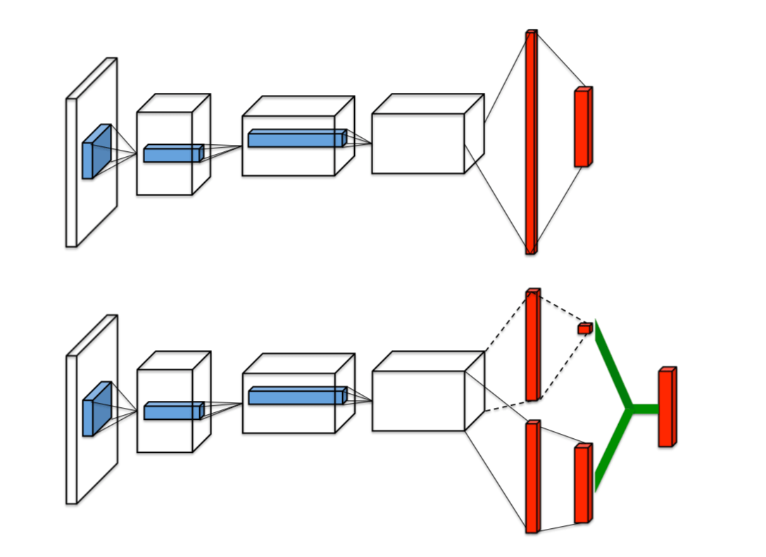
Figure 2: Contrasting Q-networks with Dueling Q-networks. Taken from the original research paper on the matter.
The top network in Figure 2 shows a normal convolutional Q-network while the bottom image show the dueling Q-network architecture defined in this section. Notice how in the bottom network, two outputs are generated (value and advantage), which are combined together to generate the normal Q-value estimation.
Note that this improvement to the original DQN framework amounts only to a simple neural architecture change. So instead of looking at the code for DDQN algorithm again lets drill down on how the neural network architecture is defined in Tensorflow for each *_estimator. To keep this simple, I’ll make this network just a bunch of fully connected layers with RELUs activations.
# Placeholders for our input
self.X_pl = tf.placeholder(shape=(None, state_dim), dtype=tf.float32, name="X")
# The TD target value
self.y_pl = tf.placeholder(shape=(None,), dtype=tf.float32, name="y")

self.weights = tf.placeholder(shape=(None,), dtype=tf.float32, name="weights")

self.actions_pl = tf.placeholder(shape=(None,), dtype=tf.int32, name="act")

batch_size = tf.shape(self.X_pl)[0]

self.fcl1 = tf.layers.dense( self.X_pl, 128, activation=tf.nn.relu, name='fcl1')

if deulling is True:
    # value prediction layers
    self.fcl2_value = tf.layers.dense( self.fcl1, 128, activation=tf.nn.relu, name='fcl2_value' )
    self.value_prediction = tf.layers.dense( self.fcl2_value, 1, name='fcl3_value')

    # advantage prediction layers
    self.fcl2_advantage = tf.layers.dense( self.fcl1, 128, activation=tf.nn.relu, name='fcl2_advantage')
    self.advantage_prediction = tf.layers.dense( self.fcl2_advantage, action_space, name='fcl3_advantage')

    self.mean_advantage = tf.reduce_mean(tf.reduce_mean(self.advantage_prediction))
    self.predictions = self.value_prediction + (self.advantage_prediction - self.mean_advantage)
else:
    self.fcl2 = tf.layers.dense( self.fcl1, 128, activation=tf.nn.relu )
    self.predictions = tf.layers.dense( self.fcl2, action_space )
Line 12: Here I define the common layer used by the advantage, state-value and vanilla Q-networks.
Lines 17-22: Here I define the branching state value and advantage networks respectively. Notice how both networks take self.fcl1 as an input into their first layers.
Lines 24-25: finally I calculate the Q-value by combining the state-value and advantage estimates. There’s one caveat though, I also subtract the mean advantage from advantage value. Why do I do this? Mostly for stability reasons as subtracting by the mean indicates that the advantage only needs to change as fast as the mean advantge over the entire batch.
Prioritized Experience Replay
The next significant improvement to the DQN framework was that of prioritized experience replay. This idea deals with assigning priorities to each of the state transitions stored in the replay buffer. These priorities are based on their TD error (
Of course, this method also has a lot of added complexity. Firstly, the replay buffer can no longer just be a simple circular buffer and sampling from the buffer can no longer be just a O(1) operation. This means new more complex data structures (i.e. sum-trees )are required to efficiently implement prioritized sampling in optimal O(log(N)) runtime. Furthermore, since experiences are no longer just drawn randomly from the replay buffer, the agent needs to incorporate importance sampling into the Q-value update operation. The use of importance sampling is required as this method requires the agent to sample from a distribution that is different from the natural distribution that generated each of the state transitions. However, the rate of importance sampling starts off very small and is greatly annealed over time. This makes sense as at the start, the agent favors exploratory actions and its policies are bound to rapidly change as a result. Hence, importance sampling only becomes crucial near convergence when unbiased updates are required
My implementation of this algorithm doesn’t use any of the fancy data structures described in the original research paper to optimize for runtime. This means it probably won’t scale for very complex RL tasks. Nevertheless, this implementation should suffice to illustrate the concept and experiment with a variety of OpenAI gym environments. There is a lot of numpy wrangling in this implementation so I won’t describe it in detail. However, those of you who are curious can still view all the code for this algorithm here. Pay special attention to the PriorityBuffer class, which implements all of the core functionality associated with prioritized sampling.
Conclusion
The DQN framework that I’ve outlined in this post is useful for most discrete action-space problems. However, significant challenges arise when you use this algorithm for problems that naturally have continuous action spaces (i.e. most robotics problems). So, how do we extend the RL framework to tackle these types of challenges? Well, thats where policy gradient methods come in, which will be the topic of the next blog post.
